Solow Growth Model

Assumptions §

• ass. Investments are equal to savings, i.e. all savings are invested. $I=S$
• ass. $Y=F(K_t,N_t,z_t)$

Intertemporal Utility Maximization §

ass. Households perform intertemporal utility maximization. Similar to Utility Maximization but according to the following general form of intertemporal utility maximization:

$$\underset{c_1,c_2}{\max }{c}_1^{\alpha }{c}_2^{1-\alpha },\forall t{C}_t+S_t=w_t{N}_t+r_t{K}_t$$

The equality is the intertemporal budget constraint that holds from $t=t_0,t_1,\dots$. Limit the time horizon to just two periods, $t$ and $t+1$. Then:

1. Capital stock is initially $K_t=0$
2. No savings at second (=last) period $S_{t+1}=0$ Then the two constraints:

• $C_t+S_t=w_t{N}_t$
• $C_{t+1}=w_{t+1}{N}_{t+1}+(1+r)S_t$ Equating for $S_t$ we get:

$$\underset{\text{ NPV }}{\underbrace{\frac{1}{(1+r)}}}\underset{\text{ Savings carried over }}{\underbrace{(C_{t+1}-w_{t+1}{N}_{t+1})}}=\underset{\text{ Save at t }}{\underbrace{w_t{N}_t-C_t}}$$

This is the intertemporal budget constraint. Now solving for $C_{t+1}$ the maximization problem for the above Cobb-Douglas Utility function to get Unconstrained Maximization:

$$\underset{C_t}{\max }{C}_t^{\alpha }\stackrel{\text{ Ct+1 }}{\overbrace{[\underset{\text{ appreciated savings }}{\underbrace{(1+r)w_t{N}_t-(1+r)C_t}}+\underset{\text{ income }}{\underbrace{w_{t+1}{N}_{t+1}}}{]}^{1-\alpha }}}$$

we get the first order condition (by optimizing the log of the utility function and getting first derivative):

$$\alpha \left(Y_t+\frac{Y_{t+1}}{1+r}\right)=C_t$$

where $Y_{\tau }=w_{\tau }{N}_{\tau }$

Capital Accumulation §

ass. Law of Motion (Capital) Capital stock is acculated and depreciated via the following equation:

$$K_{t+1}=\underset{\text{ Capital stock at t }}{\underbrace{K_t}}(1-\stackrel{\text{ depreciation }}{\overbrace{\delta }})+\underset{\text{ investment at t }}{\underbrace{I_t}}$$

Then consider $I_t=S_t=s{Y}_t$ where $s$ is the savings rate. Then

$$\begin{array}{rlrlr}{K}_{t+1}& =(1-\delta )K_t& & +\underline{szF(K_t,N_t)}& \\ & & & =N_t\left(\frac{1}{N_t}F(K_t,N_t)\right)& \text{(1) CRS}\\ & & & =N_t\left(f(k_t,1)\right)& \text{(2) Intensity}\\ & =(1-\delta )K_t+sz{N}_{t}f(k_t)& & & \\ \frac{K_{t+1}}{N_t}& =(1-\delta )k_t+szf(k_t)& & & \\ k_{t+1}\frac{N_{t+1}}{N_t}& =(1-\delta )k_t+szf(k_t)& & & \end{array}$$

thm. Law of Motion (Capital, intensive) i.e. per person:

$$\begin{array}{rl}\underset{\text{ future stock }}{\underbrace{k_{t+1}}}(1+n)& =\underset{\text{ leftover }}{\underbrace{(1-\delta )k_t}}+\underset{\text{ inflow }}{\underbrace{szf(k)}}\\ k_{t+1}& =\frac{1-\delta }{1+n}{k}_t+\frac{1}{1+n}{i}_t\end{array}$$

• $k_t:=\frac{K_t}{N_t}$ i.e. capital intensity, in $\text{(2) Intensity}$
• $n:=\frac{N_{t+1}-N_t}{N_t}$ i.e. population growth rate
• $f(k_{\tau })$ is the individual production function, i.e. per worker ($N_{\tau }=1$)
• $i_t:=szf(k_t)$, investment (=saving) in intensive form
• $\text{(1) CRS}$ works because of assumption of constant returns to scale: $\delta F(K_t,N_t)=F(\delta K_t,\delta N_t)$

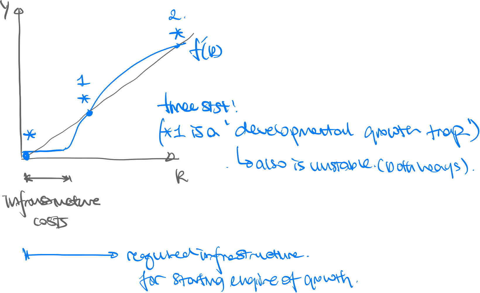
Implications §

corr. Capital change can be simply caldualted:

$$△k:=k_{t+1}-k_t=-\delta k_t+szf(k_t)$$

1. Capital accumulation cannot explain per capital GDP growth
   • …due to diminishing ${\text{MP}}_L,{\text{MP}}_K$ in $F(\cdot )$
2. Explains why per capita GDP converges to a certain point (intersection point in right graph)
3. Expalins why total GDP grows as population increases, but also that population growth does not cause per capital GDP growth

Steady State Capital §

We consider the steady state point, the intersection point in the right graph. We assume:

• $\hat{k}:=\frac{k_{t+1}-k_t}{k_t}$ i.e. capital growth rate
• $zf(k_t):=z{k}^{\alpha }$ i.e. Cobb-Douglas production function

$$\begin{array}{rl}\hat{k}& :=\frac{-\delta k_t+szf(k_t)}{k_t}\\ & =-\delta +s{k}_t^{\alpha -1}\end{array}$$

At steady state ${\hat{k}}_{\text{stst}}=0$. Thus:

$$\begin{array}{rl}\delta & =s{k}_{\text{stst}}^{\alpha -1}\\ k_{\text{stst}}& ={\left(\frac{\delta }{sz}\right)}^{1/\alpha -1}\end{array}$$

Reformulation with Productivie Hours of Labor §

let

1. $g=\frac{z_{t+1}-z_t}{z_t}$ the growth rate of $z$.
2. $\tilde{k}:=\frac{K}{zN}$ disembodied intensive capital i.e. “body-hours,” i.e. when productivity is disembodied.
   1. This also implies $\widetilde{k_{t+1}}=\frac{K_t}{z_t{N}_t(1+n)(1+g)}$ We have thm. Law of motion for disembodied capital:

$$\begin{array}{rl}\widetilde{k_{t+1}}& =\frac{1-\delta }{(1+n)(1+g)}\widetilde{k_t}+\frac{sf(\widetilde{k_t})}{(1+n)(1+g)}\\ △\widetilde{k_{t+1}}& =\frac{(1-\delta )-(1+n)(1+g)}{(1+n)(1+g)}\widetilde{k_t}+[\dots ]\end{array}$$

At steady state $△\tilde{k}=0$ i.e. ${\tilde{k}}_{t+1}={\tilde{k}}_t$ and we get:

$${\tilde{k}}_{\text{stst}}={\left(\frac{s}{n+g+\delta +ng}\right)}^{1/(1-\alpha )}$$

Dynamics §

Various Growth Rates §

Observe first that if $\tilde{k}$ can reach a steady state, then growth at the steady state is also zero:

$$\widehat{f(k)}=\hat{k}=\hat{\tilde{k}}=0$$

Denote growth rates:

• $\ln (N)=n$, population grwoth
• $\ln (z)=g$, productivity growth
• $\ln (\tilde{y})=0$, as we showed. Example.

$$\begin{array}{rl}\ln (Y)& =\ln \left(\frac{zNY}{zN}\right)=\ln \left(zN\cdot \frac{Y}{zN}\right)=\ln \left(zN\cdot \tilde{y}\right)\\ & =\ln (z)+\ln (N)+\cancel{\ln (\tilde{y})}\\ & =g+n\end{array}$$

\ln(\tilde{y})=0.

Convergence & Endogenous Growth §

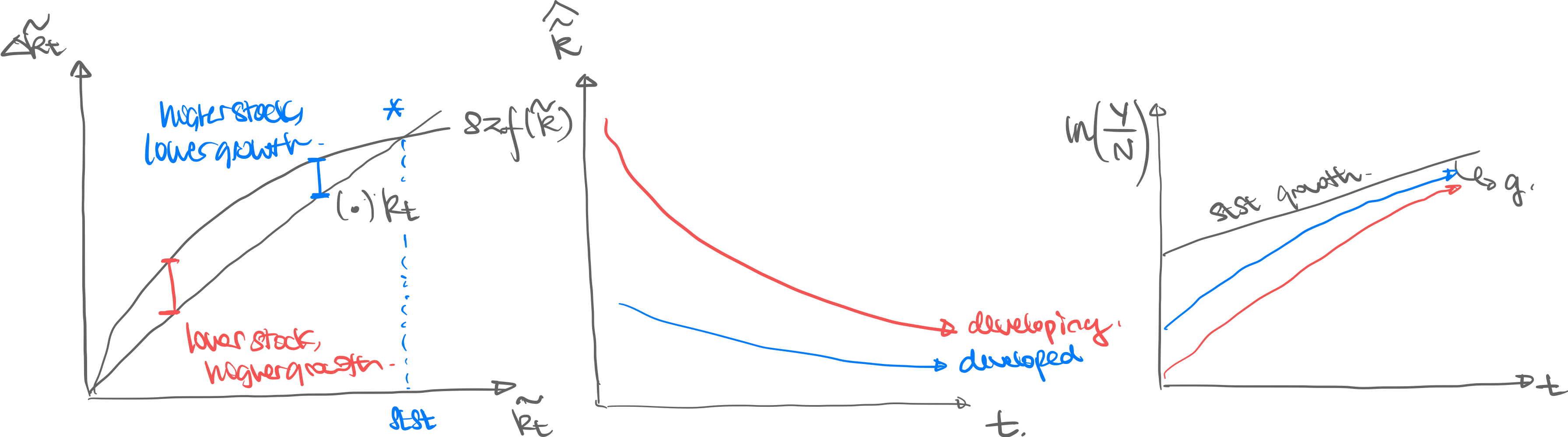
Observe.

• Red is developing, blue is developed nation.
• Reason for convergence is dinimininshing marginal product of capital ${\text{MP}}_K$

Differently-shaped Production Functions §