Better Gradient Descent Methods

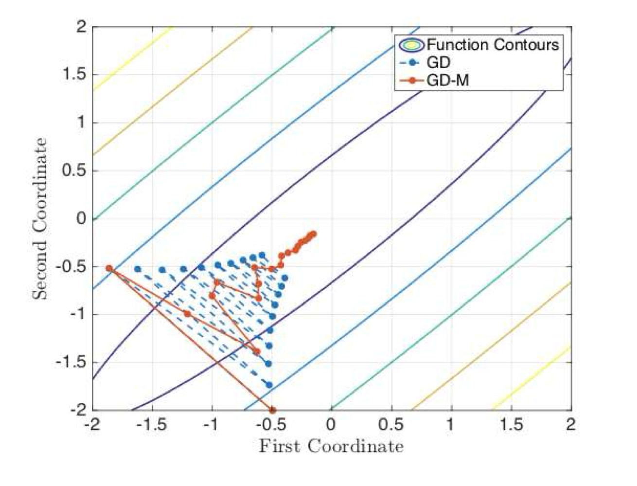
Motivation. While gradient descent is accurate it is computationally intensive. We shall consider heuristics to improve the computational speed.

def. Gradient Descent. We will use the following notation/characterization of gradient descent.

$${\mathbf{w}}_{k+1}={\mathbf{w}}_k-{\alpha }_k\left[\frac{1}{N}\sum _{i=1}^N\nabla f_i({\mathbf{w}}_{\mathbf{k}})\right]$$

where

• ${\alpha }_1,\dots ,{\alpha }_k,\dots$ are learning rates on step $k$
• $f_i$ is the loss function for datapoint $i$ and weghts ${\mathbf{w}}_{\mathbf{k}}$

Motivaiton. The first step to optimize is to avoid calculating the gradients of all datapoints $i=1,\dots ,N$.

def. Stochastic Gradient Descent. For each step, we instead randomly choose one datapoint, $j$ to update:

$${\mathbf{w}}_{k+1}={\mathbf{w}}_k-\alpha \hat{\nabla }{f}_j({\mathbf{w}}_{\mathbf{k}})$$

This works because $\underset{\text{ expectation of gradient }}{\underbrace{\mathbb{E}[\hat{\nabla }{f}_j]}}=\underset{\text{ average gradient }}{\underbrace{\frac{1}{N}\sum _{i=1}^N\nabla f_i}}$

Motivation. This is better, but this leads to lots of steps $k$. We can group or “batch” data together to reduce that, while also not calculating all gradients like classical GD. The gradient used like this, is an unbaised Estimator of the true gradient calculated over all datapoints.

def. Batch Gradient Descent. For each step, choose a random batch of size $n$, $\{j_1,\dots ,j_n\}$ and average them.

$${\mathbf{w}}_{k+1}={\mathbf{w}}_k-{\alpha }_k\left[\frac{1}{n}\sum _{i=1}^n\nabla f_{j_i}({\mathbf{w}}_{\mathbf{k}})\right]$$

Momentum §

Intuition. Momentum is a way to “dampen” the oscillations when taking many tiny steps, and to reduce the number of steps required for convergence (by a factor of a square root). This dampening, implemented for stochastic/batch gradient descent, can be considered as a bias-variance-tradeoff of the gradient estimator.

alg. Nesterov’s Accelerated Gradient Descent (NAG). This is convoluted but it’s optimized to guarantee a certain rate of convergence, see below. This is also the original implementation of momentum.

1. let ${\lambda }_0=0,{\lambda }_k=1+\frac{1}{2}\cdot \sqrt{1+r{\lambda }_{k-1}^2}$
2. let ${\gamma }_k=\frac{1-{\lambda }_k}{{\lambda }_{k+1}}$
3. for steps $k=\mathrm{1..}$, setting $w_1=t_1$:
   1. Momentum: $t_{k+1}={\mathbf{w}}_{\mathbf{k}}-\frac{1}{\beta }\nabla f_j({\mathbf{w}}_{\mathbf{k}})$
   2. Descent: ${\mathbf{w}}_{k+1}=\underset{\text{ weighted sum of momentum}}{\underbrace{(1-{\gamma }_k)t_{k+1}+{\gamma }_k{t}_k}}$

thm. (informal statement). Step $k$ will minimize:

$$\underset{\text{ distance to optimal at step k }}{\underbrace{f({\mathbf{w}}_k)-f({\mathbf{w}}^{\ast })}}\le \frac{1}{k^2}\underset{\text{ constant }}{\underbrace{2\beta ||{\mathbf{w}}_1-{\mathbf{w}}^{\ast }|{|}_2^2}}$$

i.e., the distance to optimal drops quadratically wrt $k$

alg. GD with Momentum. A more intuitive way to incorporate momentum. Setting $\beta \in [0,1]$ to how much you want to accumulate prior momentum:

1. for $k=0\dots$:
   1. Momentum: $m_{k+1}=\beta m_k+\nabla f_i({\mathbf{w}}_k)$
   2. Descent: ${\mathbf{w}}_{k+1}={\mathbf{w}}_k-\alpha m_{k+1}$

Higher-order Methods §

Intuition. Curvature is useful for gradient descent.

Adaptive Learning Rates §

Intuition. We adapt the learning rates for each parameter. Small learning rate for frequently updated parameters, and large learning rates for infrequently updated parameters. This works because:

1. Frequently updated parameters can be overfit, and infrequently updated ones underfit
2. By adjusting learning rates inversly to frequency/magnitude of update we reduce overand underfitting, while also improving convergence rates

alg. GD with Adaptive Learning Rates. (Adagrad) It is proven that it reduces regret bounds

1. for $k=0,\dots$
   1. Sum-of-Squares accumulation: $v_{k+1}=v_k+\underset{\text{ sqared gradient }}{\underbrace{\nabla f\odot \nabla f}}$
   2. Adaptive rate: ${\alpha }_k=\gamma \cdot 1/(ϵ+\sqrt{v_{k+1}})$ (element-wise divide)
   3. Descent: ${\mathbf{w}}_{k+1}={\mathbf{w}}_k-{\alpha }_k\odot \nabla f$ The sum of squares will grow fast for parameters with high gradients and/or frequent updates. The learning rate is the reciprocal, and thus diminishes. v.v.

alg. Root-Mean-Squared Propagation. (RMSprop). Adaptive learning rates using exponential moving average. Set a learning rate sequance ${\alpha }_1,\dots ,{\alpha }_k,\dots$ such that ${\alpha }_k\to 0$ at a rate $k^{1/2}$. Then:

1. for $k=0,\dots$
   1. Sum-of-Squares accumulation: $v_k+\underset{\text{ sqared gradient }}{\underbrace{\nabla f\odot \nabla f}}$
   2. Decaying SoS (=“preconditioner”) ${\mathbf{b}}_k=\gamma \cdot 1/(ϵ+\sqrt{v_{k+1}})$ (element-wise divide)
   3. Descent: ${\mathbf{w}}_{k+1}={\mathbf{w}}_k-{\alpha }_k{\mathbf{b}}_k\odot \nabla f$

Adaptive Learning Rate + Momentum §

alg. Adaptive Learning Rate with Momentum (ADAM). Integrate both the adaptive learning rate (into second moment) and momentum (first moment).

1. for $k=0,\dots$
   1. First moment: $m_{k+1}^{(1)}={\beta }_1{m}_k^{(1)}+(1-{\beta }_1)\nabla f$
      1. Debias: ${\tilde{m}}_{k+1}^{(1)}=\frac{m_{k+1}^{(1)}}{1-{\beta }_1^{(k+1)}}$
   2. First moment: $m_{k+1}^{(2)}={\beta }_1{m}_k^{(2)}+(1-{\beta }_2)\nabla f\odot \nabla f$
      1. Debias: ${\tilde{m}}_{k+1}^{(2)}=\frac{m_{k+1}^{(2)}}{1-{\beta }_2^{(k+1)}}$
   3. Descent: ${\mathbf{w}}_{k+1}={\mathbf{w}}_k-{\alpha }_k{\tilde{m}}_{k+1}^{(1)}/(ϵ+\sqrt{{\tilde{m}}_{k+1}^{(2)}})$

Conclusion

Just use ADAM.