Motivation. Let’s say that there is a relationship between GDP per capita and life expectancy. Maybe god has declared a perfect formula describing this relationship:
While we humans may never truly know the parameters of the formula, and , we can still make a good guess about it. Therefore, assuming this is a linear relationship, we have the Bivariate Ordinary Least Squares Model.
where are observations (=regressors).
thm. Parameter OLS Estimator for observations :
Properties.
- Predictor:
- Residual: is the estimator for the error term, i.e. how good the predictor is.
- Regression Variance: where is the number of parameters ( in this case)
- basically the Mean Squared Error. The lower the better.
- This is also the standard error of the residuals.
- In Stata, it’s called the
Root MSE.
Evaluation of Estimators.
- Mean of :
- Thus bias is
- If then exogenous (good!)
- If then there’s some 3rd factor positively correlated with , thus bias is positive.
- If then v.v.
- & Thus the bias characterizes exogeniety
- Variance of :
- This is also called precision
- is also called standard error of .
- ! For random variables, is called standard deviation. For estimator random variables, it is called standard error. An abuse of terminology.
Confidence Intervals and Hypothesis Testing
See also: Confidence Intervals and Hypothesis Testing
Motivation. Assume we have our estimators for our sample size using OLS, . Now, assuming we have the true population data (impossible in real life) and take samples of size from the whole population, we get different tuple of estimators . If we plot these on a graph, we get an approximate bell curve. This is due to the Central Limit Theorem. Knowing this fact, we can deduce if there is a correlation between and .
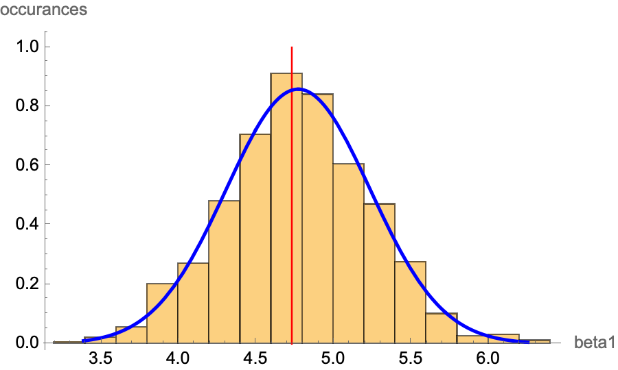
Remark. is the minimum required for CLT. is a conservative requirement for CLT to apply. Remark. We will only look at since it is the more important parameter.
Hypothesis Testing
def. The Null hypothesis in regression is , i.e. there is no correlation.
def. Regression T-test. See Student’s t-test. A T-test is a test for rejecting the null hypothesis. let the T-statistic . Then
- The cutoff value is determined by how powerful (=) you want the test to be. This is determined by the Student’s T-Distribution.
- This is because
- This is Student’s t-test but with only one random variable.
- Normally, we set the cutoff , i.e. two standard deviations away. This is around an test.
Confidence Interval
Intuition.
Bias:
standard error of regression: mean squared of residuals; also the estimator for the error
Standard error of…
- Residuals → standard error of regression
- Varaince of is also the variance of CLT limit with the same sample size
Omitted Variables
Motivation. Let’s say that there is a relationship between GDP per capita and life expectancy. Maybe god has declared a perfect formula describing this relationship:
While we humans may never truly know the parameters of the formula, and , we can still make a good guess about it. Therefore, assuming this is a linear relationship, we have the Bivariate Ordinary Least Squares Model.
where are observations (=regressors). The OLS algorithm will minimize the squared sum of residuals:
where . Note the square.
thm. Parameter OLS Estimator for observations
Properties.
- Predictor:
- Residual: is the estimator for the error term, i.e. how good the predictor is.
- i.e. the mean of residuals is zero in OLS algorithm.
- OLS results in assuming that is exogenous, i.e. .
- Regression Variance: where is the number of parameters ( in this case)
- basically the Mean Squared Error. The lower the better.
- is also the standard error of the residuals.
- In Stata, is called the
Root MSE
Evaluation of Estimators.
- Mean of :
- Thus bias is
- If then exogenous (this is the definition of exogeniety)
- If then there’s some 3rd factor positively correlated with , thus bias is positive.
- If then v.v.
- & Thus the bias characterizes exogeniety
- Variance of :
- This is also called precision
- is also called standard error of .
- ! For random variables, is called standard deviation. For estimator random variables, it is called standard error. An abuse of terminology.
Other Data when Regression is Run
There are a bunch of other variables that may matter, that is not included in the above core set of variables of the regression. Here are a few:
def. Coefficient of Determination (R-Squared). Intuition: The proportion of the variation in that can be determined from . We define it as:
where
- residual sum of squares
- total sum of squares
Example. A of means that around of the variation in is explained by . Therefore, the higher it is, the better the regression is (=has more explanatory power).
Remark. It can also be shown that:
Measurement Error
Motivation. There are measurement errors in every data; it can be both in the independent variable or the dependent variable . We can characterize measurement error (in this case a measurement error in ) as:
where is randomly distributed with and std. dev. , which is the measurement error. In this case, the regression in the model will also change, into:
We can extract a couple of facts from this relationship:
- Attenuation bias: the greater the , the closer is to zero.
- if then , i.e. no measurement error
Alternatively, if there is a measurement error in , then:
- Measurement error: where and std. dev.
- Error term is absorbed by error term
- This will increase (variance of regression) and thus , but does not bias the estimator.
Issues to Watch out for
Heteroskedasticity is when the variance of data is different for some subsets of data than other subsets. ⇒ Use heteroskedatic-consistent standard errors by using robust in stata. This does not affect value of (how!) and does not bias it.
Autocorrelation often occurs in time series data where the error terms are sticky. For example, attendance at a NY yankees game will be sticky, because people who watched a good year will probably come back next year, even if the yankees aren’t as good as the year before. → used lagged variables