Following is code used for regression:
### KELP DATA ###

# Kelp data
Length_kelp <- c(0.12, 0.56, 0.56, 0.99, 1.20, 20.90, 33.10, 12.50, 8.70, 3.40, 2.90, 16.40, 21.20, 8.90, 12.60)
Biomass_kelp <- c(21, 32, 27, 34, 45, 1456, 3752, 950, 501, 198, 167, 1275, 1987, 645, 876)
data_kelp <- data.frame(Length = Length_kelp, Biomass = Biomass_kelp)

# Linear Model for Kelp
model_kelp <- lm(Biomass ~ Length, data = data_kelp)

# Plot for Kelp with custom y-axis limits to include negative values
plot(data_kelp$Length, data_kelp$Biomass,
     main = "Biomass vs Length (Kelp)",
     xlab = "Length (m)",
     ylab = "Biomass (g)",
     pch = 19, col = "blue",
     ylim = c(-500, max(data_kelp$Biomass)))  # Set y-axis limits to include negative values

# Add regression line for Kelp model
abline(model_kelp, col = "red", lwd = 2)

# New Length values for prediction (Kelp)
new_lengths_kelp <- data.frame(Length = c(34.2, 19.8, 15.4, 0.21, 1.5))

# Predict Biomass using the kelp model
predicted_biomass_kelp <- predict(model_kelp, newdata = new_lengths_kelp)

# Combine Lengths and Predicted Biomass into a data frame
kelp_predictions <- data.frame(
  Length = new_lengths_kelp$Length,
  Predicted_Biomass = predicted_biomass_kelp
)

# Add the new predicted points to the plot
points(kelp_predictions$Length, kelp_predictions$Predicted_Biomass,
       pch = 17, col = "darkgreen", cex = 1.5)

# Add a legend to the plot
legend("topleft", legend = c("Original Data", "Regression Line", "Predicted Points"),
       col = c("blue", "red", "darkgreen"), pch = c(19, NA, 17), lty = c(NA, 1, NA))


### WHALE DATA ###

# Whale data
Length_whale <- c(3.3, 9.3, 13.2, 4.1, 11.7, 4.2, 4.5, 8.4, 8.1, 6.2, 9.6, 9.7, 3.9, 7.3, 12.2)
Biomass_whale <- c(600, 9100, 8000, 800, 9800, 2000, 1800, 7500, 4100, 5000, 9800, 9200, 700, 4000, 11800)
data_whale <- data.frame(Length = Length_whale, Biomass = Biomass_whale)

# Linear Model for Whale
model_whale <- lm(Biomass ~ Length, data = data_whale)

# Plot for Whale with custom y-axis limits to include negative values
plot(data_whale$Length, data_whale$Biomass,
     main = "Biomass vs Length (Whale)",
     xlab = "Length (m)",
     ylab = "Biomass (kg)",
     pch = 19, col = "green",
     ylim = c(-10000, max(data_whale$Biomass)))  # Set y-axis limits to include negative values

# Add regression line for Whale model
abline(model_whale, col = "purple", lwd = 2)

# New Length values for prediction (Whale)
new_lengths_whale <- data.frame(Length = c(14.1, 2.9, 2.1, 13.8, 6.2))

# Predict Biomass using the whale model
predicted_biomass_whale <- predict(model_whale, newdata = new_lengths_whale)

# Combine Lengths and Predicted Biomass into a data frame
whale_predictions <- data.frame(
  Length = new_lengths_whale$Length,
  Predicted_Biomass = predicted_biomass_whale
)

# Add the new predicted points to the plot
points(whale_predictions$Length, whale_predictions$Predicted_Biomass,
       pch = 17, col = "orange", cex = 1.5)

# Add a legend to the plot
legend("topleft", legend = c("Original Data", "Regression Line", "Predicted Points"),
       col = c("green", "purple", "orange"), pch = c(19, NA, 17), lty = c(NA, 1, NA))
Following are figures generated by the code:
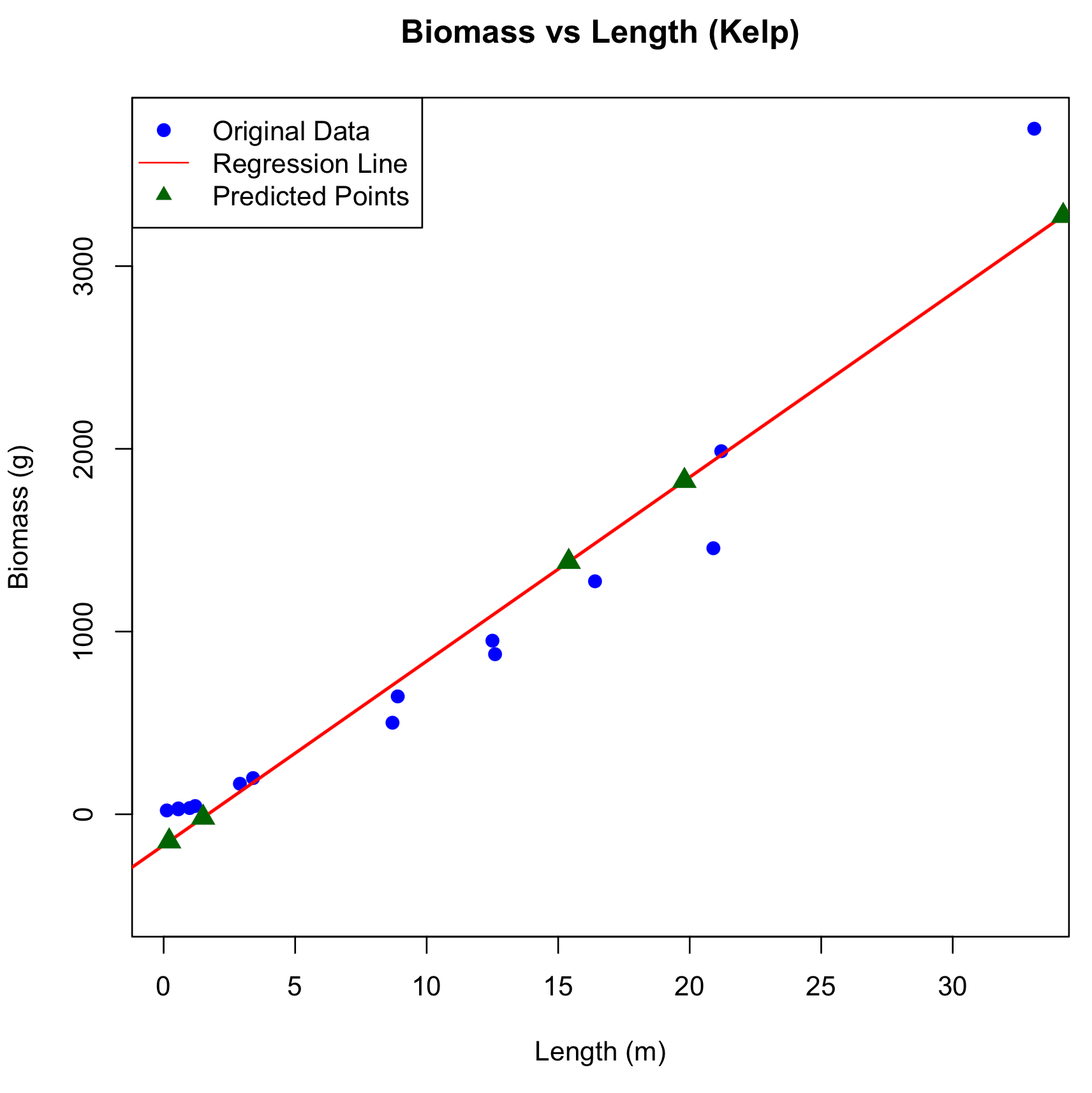
Figure 1: Relationship between Biomass and Length in Kelp
The scatter plot illustrates the relationship between Length (in meters) and Biomass (in grams) for Kelp. The blue dots represent the original dataset, with Biomass values corresponding to various Lengths. The red line is the linear regression line fitted to the data, indicating the estimated relationship between Length and Biomass. Green triangles show the predicted Biomass values for new Length inputs based on the regression model. The x-axis represents Length (m), and the y-axis represents Biomass (g).
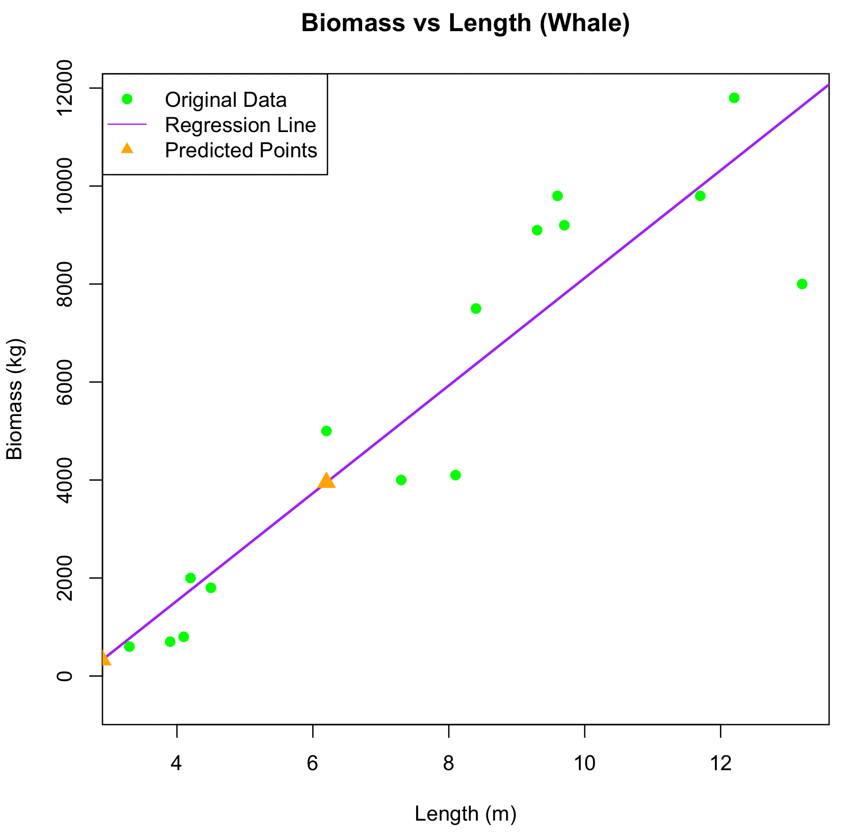
Figure 1: Relationship between Biomass and Length in Whales
This scatter plot illustrates the relationship between Length (m) and Biomass (kg) for Whales. The green dots represent the original dataset, with Biomass values corresponding to various Lengths. The purple line is the linear regression line fitted to the data, showing the estimated relationship between Length and Biomass. Orange triangles show the predicted Biomass values for new Length inputs, based on the regression model. The x-axis represents Length (m), and the y-axis represents Biomass (kg).
> summary(model_kelp)

Call:
lm(formula = Biomass ~ Length, data = data_kelp)

Residuals:
   Min     1Q Median     3Q    Max
-479.6 -172.8   24.9  121.8  587.7

Coefficients:
            Estimate Std. Error t value Pr(>|t|)
(Intercept) -169.328     92.746  -1.826   0.0909 .
Length       100.715      6.858  14.687 1.79e-09 ***
---
Signif. codes:  0 ‘***’ 0.001 ‘**’ 0.01 ‘*’ 0.05 ‘.’ 0.1 ‘ ’ 1

Residual standard error: 253 on 13 degrees of freedom
Multiple R-squared:  0.9432,	Adjusted R-squared:  0.9388
F-statistic: 215.7 on 1 and 13 DF,  p-value: 1.791e-09

> summary(model_whale)

Call:
lm(formula = Biomass ~ Length, data = data_whale)

Residuals:
    Min      1Q  Median      3Q     Max
-3638.8  -785.3  -166.6  1196.0  2114.7

Coefficients:
            Estimate Std. Error t value Pr(>|t|)
(Intercept)    -2858       1092  -2.618   0.0213 *
Length          1098        131   8.382 1.34e-06 ***
---
Signif. codes:  0 ‘***’ 0.001 ‘**’ 0.01 ‘*’ 0.05 ‘.’ 0.1 ‘ ’ 1

Residual standard error: 1599 on 13 degrees of freedom
Multiple R-squared:  0.8439,	Adjusted R-squared:  0.8319
F-statistic: 70.26 on 1 and 13 DF,  p-value: 1.337e-06
1. Scatterplots with Regression Lines, Equations, R², and P-values
For the Kelp regression, the equation is:
- R² value: 0.9432
- p-value: 1.79e-09 (for length parameter estim.) For the Whale regression, the equation is:
- R² value: 0.8439
- p-value: 1.34e-06 (for length parameter estim.)
2. Predict the Biomass for the New Samples
Kelp
  Length Predicted_Biomass
1  34.20         3275.1112
2  19.80         1824.8209
3  15.40         1381.6766
4   0.21         -148.1782
5   1.50          -18.2564
Whales
  Length Predicted_Biomass
1   14.1        12627.1889
2    2.9          327.3169
3    2.1         -551.2454
4   13.8        12297.7281
5    6.2         3951.3863
3. Interpretation of R² and P-values
- R² Value: The R² value, also known as the coefficient of determination, indicates the proportion of the variance in the dependent variable (Biomass) that is predictable from the independent variable (Length). For example, in the Kelp regression, an R² of 0.9432 means that approximately 94.32% of the variation in Kelp biomass is explained by its length. A higher R² value suggests a better fit of the model to the data.
- p-value: The p-value assesses whether the relationship observed between Length and Biomass is statistically significant. A small p-value (typically less than 0.05) indicates strong evidence against the null hypothesis (which posits no relationship between Length and Biomass), meaning that the observed relationship is unlikely to have occurred by chance. In both the Kelp and Whale models, the p-values are very small (1.79e-09 and 1.34e-06), suggesting that Length is a statistically significant predictor of Biomass for both organisms.
4. Predicting with Regression Equations vs. Using the Mean
- Regression vs. Mean: The regression equations provide a more precise and tailored prediction for Biomass based on the specific length of each organism, whereas using the mean Biomass only provides a general estimate for all organisms, irrespective of their length.
- Why Regression is Better: The regression models account for the relationship between Length and Biomass, which is especially important because Biomass tends to increase with Length in a non-linear fashion. Using the mean would ignore this relationship, leading to less accurate predictions. The high R² values in both models (94% for Kelp and 84% for Whale) indicate that Length is a strong predictor of Biomass, making regression the superior method for making predictions in this case. While the negative predicted biomasses doesn’t make sense, it can be safely ignored in this case, using other (possibly non-linear) models in order for a realistic prediction.