Consumer Surplus

Consumer Surplus §

Marginal Willingness to Pay Curve leads naturally to the concept of consumer surplus. Follow the following line of logic:

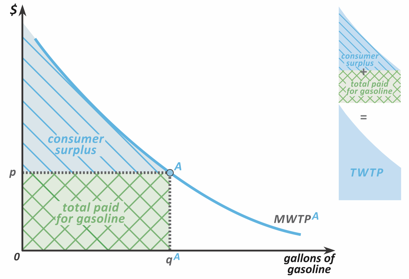
1. The area under the MWTP curve is the Total Willingness to Pay (TWTP)—the amount the consumer was willing to pay to get $q$ amount of goods.
2. Since they didn’t have to actually pay that amount (they only paid $p\times q$), they’re better off.
3. The quantitative amount that they’re better off is the Consumer Surplus

Deadweight Loss due to Taxation, Analyzed with MWTP Curves §

Consier a distortionary tax on housing prices, per square feet. The blue line shows the price $p$ per sqft of housing. The red line shows the post-tax budget line, and $A$ is the optimal point.

• → What if instead the government took away a lump sum instead of a distortionary tax? The amount taken away is $L$ and the green line shows the new budget. In this hypothetical, ideal case, the optimal is $B$.
• → In this case, the distortionary tax collected for bundle $A$ is vertial distance $T$. As $\text{DWL}:=L-T$, the vertical distance shows the Deadweight Loss for the taxation. (The lump sum was better.)

Alternatively, consider graphing the MWTP for utility $u^A$, using points $A,B$.

• → With the distortionary tax—optimal bundle: $A$, $CS=a$. Govn’t revenue is $T=h\times (p+t)=b$
• → With the lump sum tax—optimal bundle: $B$, $CS=a+b+c$

How come the consumer has more surplus as $B$ in the bottom graph? Aren’t they indifferent in MWTP?

• → The consumer instead lost the collected lump sum tax, $L$; $\therefore L=(a+b+c)-(a)=b+c$
• → ∴ $DWL=L-T=(b+c)-(b)=c$