Motivation 1. Consider the Logistic Model for classification. We observe the limitations of this model as:
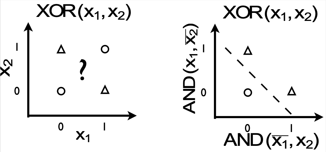
- The decision boundaries are linear, and thus can only solve linearly separable problems.
- Specifically: it can simulate OR, AND logic gates…

- …but it can’t simulate XOR because it’s not linearly separable.
- Specifically: it can simulate OR, AND logic gates…
- As seen here, we haven’t considered how to transform the ‘input space’ into the ‘feature space.’ This means we still perform terribly without this ‘magic,’ even as simple as classifiying digits in MNIST. Motivation 2. Consider how the logistic model, with its weights and bias, can be hooked up together. This resemples the neural connections of the human brain.
Feed Forward Neural Network
def. Neural Network. A feed forwarnd neural network connects the operations of multiple Logistic Models (=neurons) together.
Notation of quantities are as follows:
Let the no. of neurons (=dimensions) of each of the layers be, from the input layer: . The components of the neural net are:
- Input neurons in input space (layer ) →
- Hidden neurons (layer ) →
- Output later neuron (layer )
→
The parameters of the neural net are:
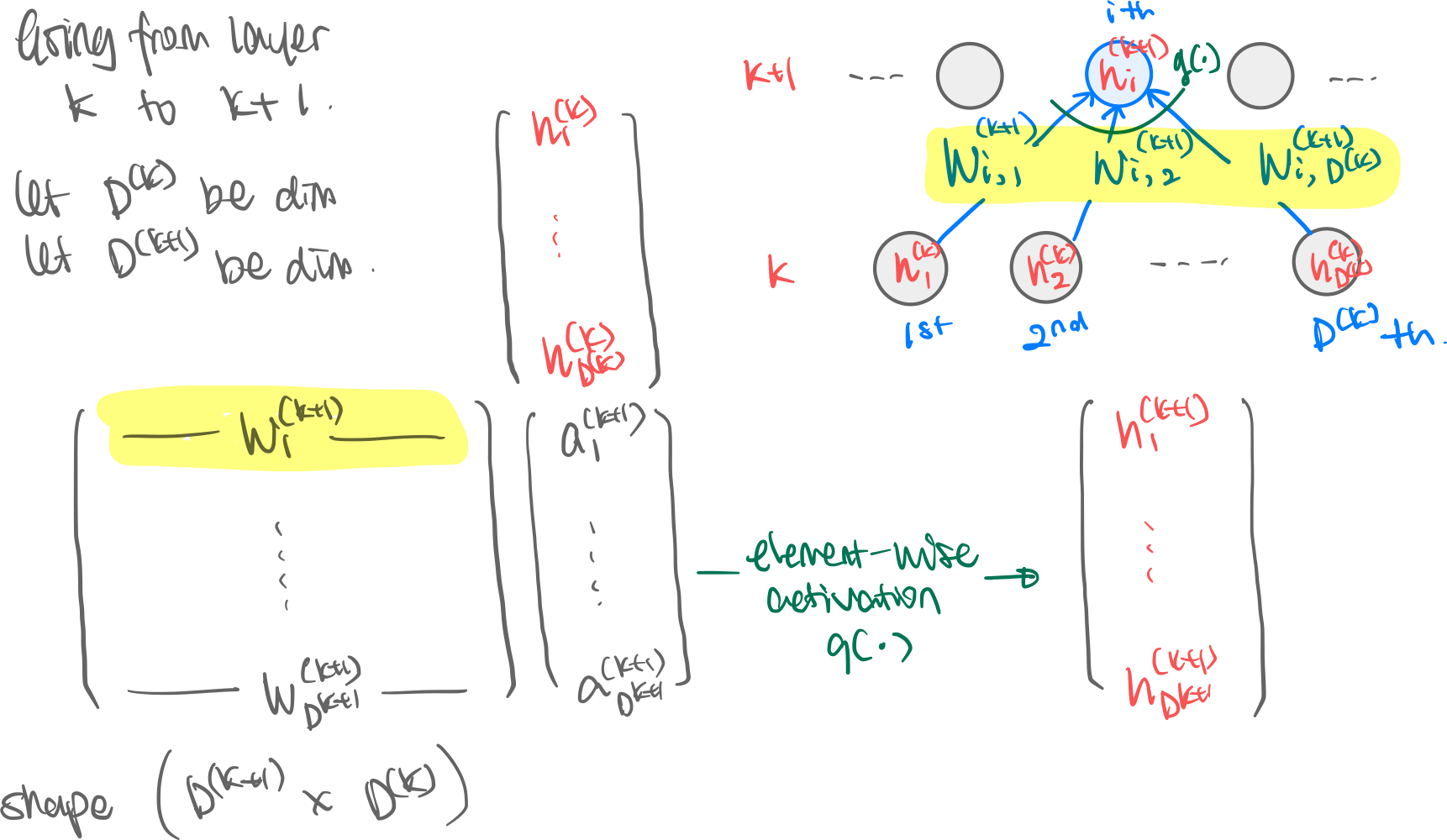
Weight parameters. Layer ’s outgoing weights are packaged into a nice matrix with shape , where refers to the weight connecting neuron in layer to neuron in layer . (This backward-ness of the indexing comes from the matrix multiplication shown later.)
Bias parameters. Layer injects a bias, into each of the neurons in layer . In matrix multiplication terms this is simply multiplying by one, as it is thusly shown in the image.
Activation Function. Each neuron in layer , having gotten its weighted input sum passes through an activation function. Without this activation function the whole NN will collapse into a simple linear map.
Visualization. The following visualization lacks the bias term for simplicity.
Mathematical Backing
Intuition. Why is this supposedly random arrangement of logistic neurons so effective expeirmentally? Here is a possible reason: neural networks can simulate any function.
thm. Universal Approximation (non-rigorous statement). Given enough depth and width, and given “normal” activation functions (sigmoid, tanh), a neural network can simulate any function to arbitrary precision.
Backpropagation
Motivation is simple. How do we find ? To do that we must minimize the loss function, i.e. find the gradient of the loss function.
def. Loss Minimization of a NN. Let NN be function is the loss of the neural network with parameters . Given training data and label The optimal parameters are:
Choice of loss function
While we can choose any loss function, from now on we will simply use the cross-entropy. similar to the loss function here, but only with one data so the second summation disappears.
For the loss function we have:
where we let as above.
def. Gradient Descent. When a analytic solution is not possible, we can minimize a function (=loss function) by numerical methods:
- Randomly select parameters
- ? Find the gradient of the loss function with one training example
- Move a little bit (, learning rate) in the direction of the gradient
- Repeat for every training example The question then is how to calculate from step 2. Here we use backpropagation:
alg. Backpropagation. We can derive the formulae for the derivatives using the chain rule. First, on the last layer : 1
then for the previous layer : 2
While we can extract the differentials wrt by:
And extract the differentials wtr by:
We can continue this until necessary according to the following visualization.
Visualization. 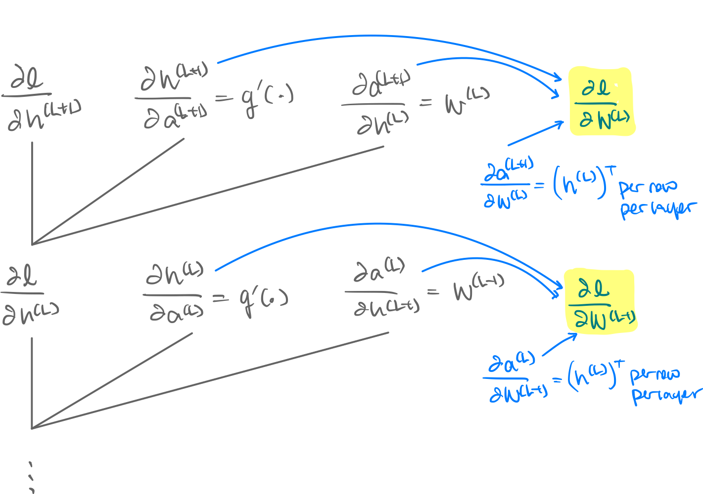
def. Gradient Descent. A form of optimization. Average the gradient of all the datapoints.
where is a chosen learning rate.
Footnotes
-
Deep Learning Slides ^9wnois ^qrkwvn ^ek9eg9 ^bvhuk5 ^bgjjby ^1t1avf ^p87mcc ^xibkdm ↩