Uncompensated Demand curve

Abstract

• The canonical, standard demand curve when we normally say “demand of good $x$”
• In theory, it should be the actual demand curves of individuals
• All Marshalian demand curves are HD0 in $(\text{prices},\text{income})$

How to Derive OPDC §

Visually:

1. Plot the indifference map and budget line for goods $x_1$ and x_2=\text{"\ of other goods”}$.Chooseanoptimalbundle$x_1$atprice$p_1$.Plotthisontheprice-quantitygraph:$A(x_1,p_1)$
2. Change the price $p_1\to p_1^{\prime }$; i.e. change the gradient of the budget. See what substitution and income effects it produces.
3. Then find the optimum bundle for the new price: $C(x_1^{\prime },p_1^{\prime })$. Connect these points together.

Analytically:

1. ${\text{max}}_{x_1,x_2}u(x_1,x_2)\text{such that}I=p_1{x}_1+p_2{x}_2$ using Utility Maximization
2. you will get $x_1(p_1,p_2,I),x_2(p_1,p_2,I)$
   1. i.e. quantity demanded as a function of prices and income
   2. This is the demand function → plot this to get demand curve

As stated above: OPDC must be HD0; check if it is!

Analysis of Goods §

• In a demand curve, Price is the negative gradient of the budget line. ($\because g=-\frac{p_1}{p_2}$, and we defined p_2=\1$)

Depending on Price §

$$\frac{\partial x_1}{\partial p_1}\begin{array}{rl}>0& ⟹\text{Ordinary Good}\\ <0& ⟹\text{Giffen Good}\end{array}$$

• Ordinary goods’s demand functions $x_1$ are homogenous in $(p_1,p_2,I)$
  • → Inflation in all prices as well as income doesn’t change anything

Depending on Income §

$$\frac{\partial x_1}{\partial I}\begin{array}{rl}>0& ⟹\text{Normal Good}\\ =0& ⟹\text{Quasilinear Good}\\ <0& ⟹\text{Inferior Good}\end{array}$$

• Graph (a) shows a normal good’s OPDC.
• Graph (b) and (c) shows a inferior good’s OPDC.
• Graph (c) is the strange Giffen Good.

Labor Supply Curve §

See also Utility Maximization with Endowments

Deriving the Labor Supply Curve works similarly to the OPDC, with the following differences:

• $p_1$ = (gradient of budget line) = (opportunity cost of leisure in dollars) = $\ast \ast w$ (wage)**
• There’s no exogenous income. You’re endowed a bundle with zero consumption and certain hours of leisure.
  • → You can “sell off” your leisure hours at price $w$

Thus as wages increase (= price of leisure in dollars)

• → the shift in the budget line happens from blue→pink in graph below…
  • …with a stationary leisure endowment at the x-intercept and a clockwise rotation.
• Then after you draw the OPDC for leisure, you flip the curve horizontally. (since $\text{endowment}=\text{leisure hours}+\text{work hours}$.)

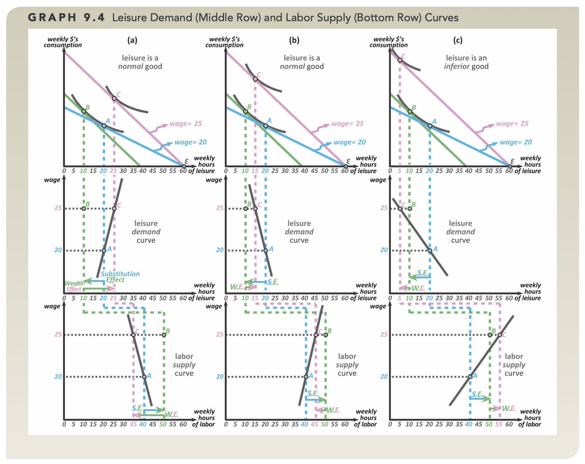
• Graph (a) shows the case where leisure is a normal good, but IE > SE.
• Graph (b) is Normal good, IE < SE.
• Graph (c) shows when leisure is an inferior good.

Warning

When discussing labor supply, the Income Effect (IE) is called the wealth effect (WE). We’re not discussing why.

Backward Bending Supply of Labor §

In real life, labor supply curves look like this:

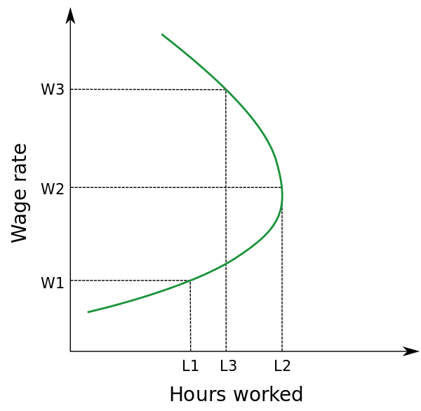
This is because workers will trade-off leisure and work hours.

→ the higher the person’s wage, they will work more; but at some point their wage is large enough and they start to enjoy life more. This is called the Backward Bending Supply of Labor.

Interesting IRL Analysis §

cdixon | How bundling benefits sellers and buyers

Deriving Uncompensated Demand §