Stochastic Process

def. Filtration on a probability space is $(\Omega ,\mathfrak{F},\{{\mathcal{F}}_t{\}}_{t\ge 0},\mathbb{P})$ where filtration $\{{\mathcal{F}}_t{\}}_{t\ge 0}$ is an increasing collection of $\sigma$-algebras where:

$$\text{for }s\le t,{\mathcal{F}}_s\subseteq {\mathcal{F}}_t$$

Example. Consider a two-step coin-flip.

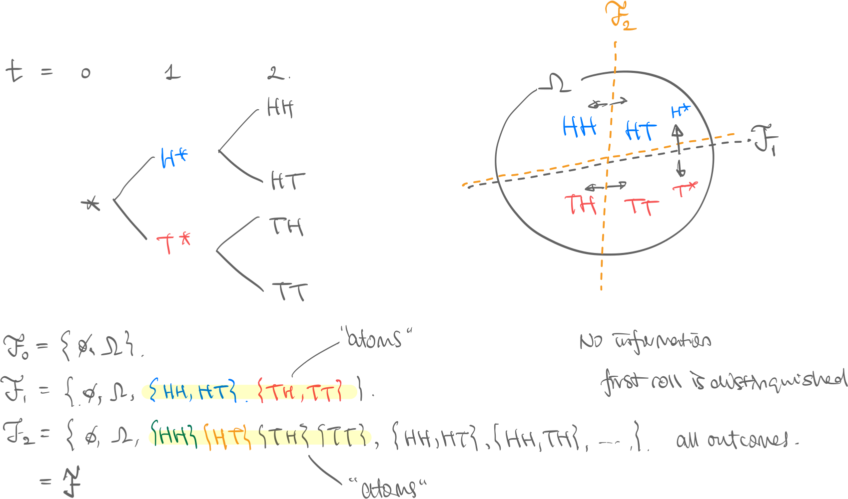
1. $\omega \in \Omega$ are the final future outcomes, HH, HT, TH, or TT.
2. ${\mathcal{F}}_1$ “cut” the outcomes in half, and now we know if we’re in the blue universe (first roll is heads) or the red universe (first roll is tails)
3. ${\mathcal{F}}_2$ “cut” the outcomes again into quarters, and now we know specifically what happened.
4. Visualization. See the pie cutting diagram. Obviously, ${\mathcal{F}}_1\subset {\mathcal{F}}_2$ because if we know the final outcome, we know if the first roll was heads or tails. Rigorously, since $\sigma$-algebras need to be closed under union, all “lower resolution” events are contained within the “higher resolution” event.

def. Adapted process = Natural Filtration. Process $\{X_t{\}}_{t\ge 0}$ is adapted to filtration $\{{\mathcal{F}}_t{\}}_{t\ge 0}$if $X_t$ is ${\mathcal{F}}_t$-measruable for every $t$. Or vice versa, the filtration is the natural filtration of the process. Example. In the above coin-flip example, let random variables $X_0,X_1,X_2$ be:

$$\begin{array}{rlr}{X}_0& =1\text{ for all outcomes}& \equiv \mathbb{E}[X_0|{\mathcal{F}}_0]\\ X_1& =\{\begin{array}{ll}2& \text{if first roll heads}\\ 3& \text{if first roll tails}\end{array}& \equiv \mathbb{E}[X_1|{\mathcal{F}}_1]\\ X_2& =\{\begin{array}{ll}4& \text{if HH}\\ 5& \text{if HT}\\ 6& \text{if TH}\\ 7& \text{if TT}\end{array}& \equiv \mathbb{E}[X_2|{\mathcal{F}}_2]\end{array}$$

Then we can easily see $X_i$ is ${\mathcal{F}}_i$-measurable, and that this process is adapted to the filtration (=filtration is the natural filtration for process $X$).

thm. From the adapted=natural process-filtration definition and the filtration definition, we have that filtration $\{\mathcal{F}\}$:

$${\mathcal{F}}_t=\sigma (X_0,\dots ,X_t)$$

• ! $\sigma (X_t)\ne {\mathcal{F}}_t$, because the former just knows about the current $X_t$, and the latter knows about all the past $X_1,\dots ,X_t$ thus ${\mathcal{F}}_t=\sigma (X_0,\dots ,X_t)$. This becomes important in the Markov property.

def. Time Series is a stochastic process indexed by discrete (integer) time points.

• See discussion: Is a time series the same as a stochastic process? - Cross Validated Example. Process $\{S_t{\}}_{t=0,1,\dots }$where it is sum of the sequence of random variables: $R_1,\dots ,R_n$:

$$S_k=\{\begin{array}{ll}{\sum }_{i=1}^k{R}_i& \text{if }k>0\\ S_0& \text{if }k=0\end{array}$$

Memoryless, True Fair-Game §

def. Martingale. A process $\{X_t{\}}_{t\ge 0}$ is a martingale iff $\text{for }s<t$

$$\mathbb{E}[X_t|{\mathcal{F}}_s]=X_s$$

Intution. True Fair-game process is a martingale. This doesn’t mean fair game in that when you begin the game, there is no unfair advantage/disadvantage (false fair-game), but that it is a fair game at every single point in time where you roll.

def. Standard Markov. A process $\{X_t{\}}_{t\ge 0}$ is a Markov process iff for $s<t$

$$\mathbb{P}(X_t\le a|\sigma (X_0,\dots ,X_s))=\mathbb{P}(X_t\le a|\sigma (X_s))$$

Intuition. Path-agnostic process is Markov. This means that giving the path of how you got to current point $s$ doesn’t matter to how the future behaves. Motivation. A process being a Markov process is a really powerful statement since we can use the relatively computationally less complex tools of Markov Chains for analysis. thm. If for process $\{X_t{\}}_{t\ge 0}$, for every $s\le t$, $\sigma (X_s)\subseteq \sigma (X_t)$ holds then it is a Markov process. $\forall s\le t$, $\sigma (X_s)\subseteq \sigma (X_t)$ is not trivial, because natural filtration contains full past history. This property holding means that current state $X_t$ encodes the past state completely, which is not necessarily true. See the Random walk with drift example.

Examples. Consider these four games:

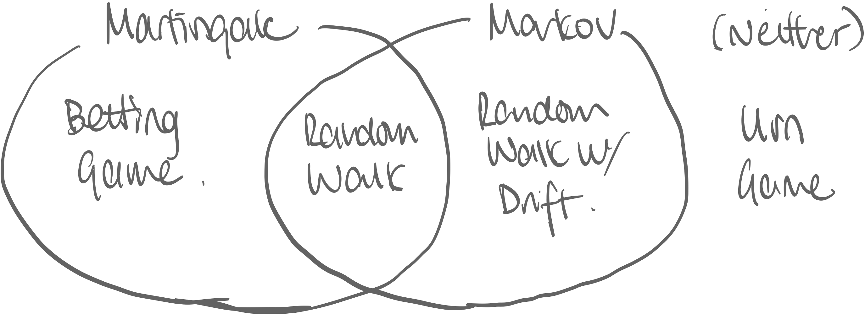
Urn Game §

Example. Two red balls and two black balls are in an urn. You pick a ball without replacement for four times. $\{C_t{\}}_{t=1,2,3,4}$ where $C_i$ is $1$ if $i$-th pick is red, and $0$ if black.

Not Markov §

$$\mathbb{P}(C_3=1|{\mathcal{F}}_2)=\{\begin{array}{ll}0& \text{if}\{RR\ast \}\\ \frac{1}{2}& \text{if}\{RR\ast \}\\ 1& \text{if}\{RR\ast \}\end{array}$$

but

$$\begin{array}{rlr}\mathbb{P}(C_3=1|\sigma (C_2))& =\{\begin{array}{llc}\mathbb{P}(C_3=1|\{\ast R\ast \})& \text{if }\{\ast R\ast \}& (1)\\ \mathbb{P}(C_3=1|\{\ast B\ast \})& \text{if }\{\ast B\ast \}& (2)\end{array}& \\ & & \\ (1)& =\mathbb{P}(C_3=1|\{BR\ast \})\cdot \mathbb{P}(C_1=1|C_2=R)& \\ & +\mathbb{P}(C_3=1|\{RR\ast \})\cdot \mathbb{P}(C_1=1|C_2=R)& \\ & =\left(\frac{1}{2}\cdot \frac{2}{3}\right)+\left(0\cdot \frac{1}{3}\right)=\frac{1}{3}& \text{Use Bayes’ Rule}\\ (2)& \text{ is computed similarly}=\frac{2}{3}& \end{array}$$

Thus $\mathcal{L}(C_3|{\mathcal{F}}_2)\stackrel{d}{\ne }\mathcal{L}(C_3|\sigma (C_2))$, meaning their distributions are not the same, and thus not path agnostic.

Not Martingale §

$$\mathbb{E}[C_2|{\mathcal{F}}_1]=\{\begin{array}{ll}\mathbb{E}[C_2|\{B\ast \}]=\frac{2}{3}& \text{if }\{B\ast \}\\ \mathbb{E}[C_2|\{R\ast \}]=\frac{1}{3}& \text{if }\{B\ast \}\end{array}$$

but

$$C_2=\{\begin{array}{ll}1& \text{if }\{\ast B\ast \}\\ 0& \text{if }\{\ast R\ast \}\end{array}$$

Thus trivially not martingale.

Betting Game §

Example. Player wins or loses on each round $i$, but depending on if they won or lost the previous round $i-1$ they bet more or less, and thus on this round $i$ the payoff changes.

$$\begin{array}{rlr}{X}_n& =X_{n-1}+b_n{R}_n& \\ & =X_0+R_0{R}_1+\cdots +R_{n-1}{R}_n& \text{since }{b}_n=R_{n-1}\end{array}$$

where

$$\begin{array}{rl}{b}_n& =\{\begin{array}{llc}2& \text{if }{R}_{n-1}=1& \text{cocky}\\ 1& \text{if }{R}_{n-1}=0& \text{insecure}\end{array}\\ R_n& =\{\begin{array}{ll}1& p=\frac{1}{2}\\ -1& p=\frac{1}{2}\end{array}\end{array}$$

Not Markov §

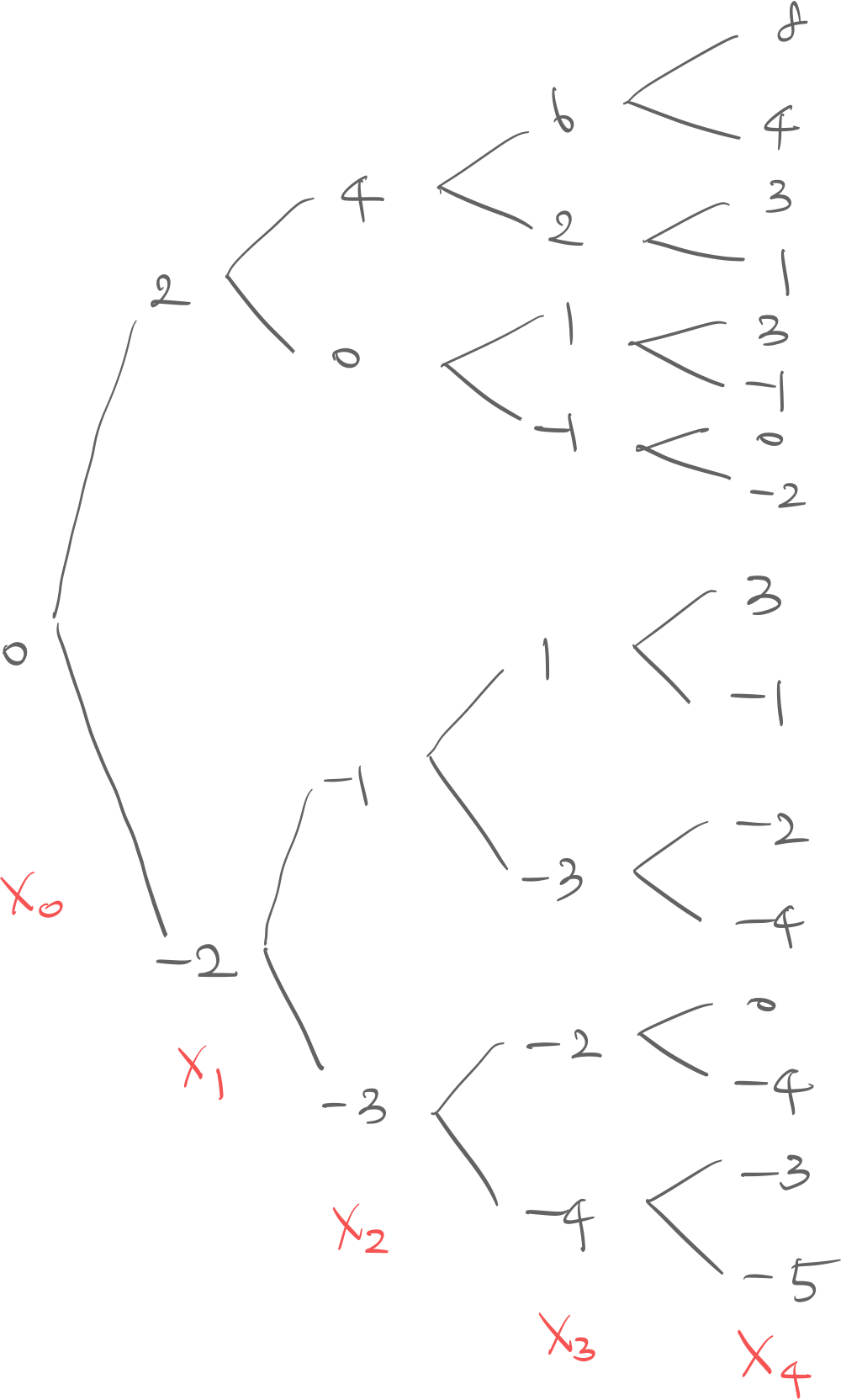
Consider the game tree. Simply observe the distribution of $X_3$ and see how well it predicts $X_4$:

• $\mathcal{L}(X_4|{\mathcal{F}}_3)$ has $2^3$ cases for each path
• $\mathcal{L}(X_4|\sigma (X_3))$ has $7$ cases since $101\ast$ and $011\ast$ both equal $1$

Is Martingale §

$$\begin{array}{rl}\mathbb{E}[X_t|{\mathcal{F}}_s]& =\mathbb{E}[X_0+R_0{R}_1+\cdots +R_{s-1}{R}_s+R_s{R}_{s+1}+\cdots +R_{t-1}{R}_t|{\mathcal{F}}_s]\\ & =\underset{X_s}{\underbrace{X_0+\cdots +R_{s-1}{R}_s}}+\cancel{R_s\mathbb{E}[R_{s+1}]+\mathbb{E}[R_{s+1}{R}_{s+2}]+\cdots }\\ & =X_s\end{array}$$

since $\mathbb{E}[R_s{R}_{s+1}]=0$ because

$$R_s{R}_{s+1}=\{\begin{array}{ll}1\cdot 1& p=\frac{1}{4}\\ 1\cdot -1& p=\frac{1}{4}\\ -1\cdot 1& p=\frac{1}{4}\\ -1\cdot -1& p=\frac{1}{4}\end{array}$$

Random Walk with Drift §

Example. Consider process $\{X_t{\}}_{t=0,1,\dots }$ where:

$$\begin{array}{rl}{X}_n& =X_{n-1}+R_n+0.1\\ & =X_0+R_1+\cdots +R_n+0.1n\\ & \\ R_n& =\{\begin{array}{ll}1& p=\frac{1}{2}\\ -1& p=\frac{1}{2}\end{array}\end{array}$$

Is Markov §

$$\begin{array}{rlr}\mathbb{P}(X_{n+1}\le a|{\mathcal{F}}_n)& =\mathbb{P}(X_n+R_{n+1}+0.1\le a|{\mathcal{F}}_n)& \\ & =\mathbb{P}(R_{n+1}\le \underset{\text{ all known under Fn }}{\underbrace{a-X_n-0.1}}|{\mathcal{F}}_n)& \\ & =\mathbb{P}(R_{n+1}\le a-X_n-0.1)& \text{since Rn+1⊥Fn }\end{array}$$

Isn’t Martingale §

$$\mathbb{E}[X_2|{\mathcal{F}}_1]=\{\begin{array}{ll}1.2& \text{if }\{1\ast \}\\ -0.8& \text{if }\{0\ast \}\end{array}$$

but

$$X_1=\{\begin{array}{ll}1.1& \text{if }\{1\ast \}\\ -0.9& \text{if }\{0\ast \}\end{array}$$

each case is off by $0.1$ due to drift.

• $R_i$ are identically distributed.: Stationary

• $E(W_{k+1}|W_1\dots W_k)=W_k$ then: Martingale

• $P(W_{k+1}=w_{k+1}|W_1=w_1,\dots W_k=w_k)=P(W_{k+1}=w_{k+1}|W_k=w_k)$: Markov

  random variable - Why do stochastic processes involve time? - Cross Validated

Strong Markov Property §

Motivation. Consider the following special Markov Chain with just two states, 0,1 and deterministic transitions:

• If at $0$, next step is $1$
• If at $1$, next step is $0$ except:
  • on the first time it arrives, it stays there for one more timestep. Thus discrete process $\{X_t\}$ has distribution:

$$X_{t+1}=\{\begin{array}{llc}1& \text{if }{X}_t=0& \\ 0& \text{if }{X}_t=0,t\ne 1& \\ 1& \text{if }{X}_t=0,t=1& \text{Special case}\end{array}$$

This is standard markov, because $X_{t+1}$ only considers $X_t$, the current step. But doesn’t it feel weird that the process depends on what timestep it is on? Shouldn’t a true memorlyless process be independent even of what time it is? def. Stopping Time. Let $\{{\mathcal{F}}_t\}$ filtration adapted to process $\{X_t\}$. A random variable $T=0,1,\cdots <\infty$ is a stopping time wrt $\{{\mathcal{F}}_t\}$ iff:

$$\{T=n\}\in {\mathcal{F}}_n$$

Intutition. Consider stopping time of the first time process its state $i$, ie $T=\min \{n\ge 1|X_{n=i}\}$. Then $\{T=n\}\in {\mathcal{F}}_n$, i.e. at time step $n$ filtration ${\mathcal{F}}_n$ is enough to show it’s time to stop. Example.

• Valid: “Stop after exactly 10 iterations”, “Stop the first time state is 10”
• Invalid: “Stop at the biggest value ever” (Impossible), “Stop when the next state is 10” (Impossible) def. Strong Markov. Let $T$ be some stopping time of your choice on process $\{X_t\}$ Then $\{X_t\}$ has the strong markov property iff for $\forall t$:

$$\underset{\text{ Process starting from t=0 }}{\underbrace{\mathcal{L}(X_{T+t}|{\mathcal{F}}_T)}}=\underset{\text{ Process starting at T }}{\underbrace{\mathcal{L}(X_t|X_0=X_T)}}$$

Intuition. Like in the motivation section, the distribution of $X_t$ at any timepoint should be independent of the timestep $t$ it is in.

Weiner Process §

Standard Weiner Process §

Motivation. Assume there are random variables $X_1\dots$ as:

$$X_i=\{\begin{array}{ll}\frac{1}{\sqrt{n}}& 0.5\text{ probability}\\ -\frac{1}{\sqrt{n}}& 0.5\text{ probability}\end{array}$$

1. let $W_k$ be a stochastic process such that:

$$W^{(n)}(t)=\{\begin{array}{ll}0& \text{if }t=0\\ R_1+\cdots +R_t& \text{if}t\in \mathbb{N}\\ \text{affine extension on closest interval }& \text{else}\end{array}$$

Then we get the Weiner process as:

$$\mathfrak{B}(t)=\underset{n\to \infty }{\lim }{W}^{(n)}(t)$$

def. Brownian Motion. (=Weiner process) $\mathfrak{B}(t)$ (written as ${\mathfrak{B}}_t$) is a set of random variables continuous-time indexed and has the following properties:

1. Is a continuous process
2. ${\mathfrak{B}}_0=0$
3. ${\mathfrak{B}}_t-{\mathfrak{B}}_s{\sim }_{d}N(0,t-s)$
   1. Thus, ${\mathfrak{B}}_t{=}_d\mathcal{N}(0,t)$
4. Any interval ${\mathfrak{B}}_a-{\mathfrak{B}}_b$ and ${\mathfrak{B}}_c-{\mathfrak{B}}_d$ where $[a,b]$ and $[c,d]$ do not overlap is independent. Notation wise, we think of $\mathfrak{B}=\{{\mathfrak{B}}_t{\}}_{t\ge 0}$, i.e. a set of random variables indexed by $t$.

Remark. Brownian Motion can also be defined as an Ito Process that satisfies the following stochastic differential equation:

$$d\mathfrak{B}=\mu \cdot dt+{\sigma }^{2}d\mathfrak{B}$$

Trivially, in the case of standard brownian motion, $\mu =0,{\sigma }^2=1$ Thus $d\mathfrak{B}=0\cdot dt+1\cdot d\mathfrak{B}$.

Properties. Brownian Motion satisfies the following properties:

• Martingale Property: Brownian motion is martingale: $\forall s\le t,\mathbb{E}({\mathfrak{B}}_t|{\mathcal{F}}_s)={\mathfrak{B}}_s$ where ${\mathcal{F}}_s=\sigma ({\mathfrak{B}}_s)$
• Markov Property:
  • $\forall s\ge 0,\{{\mathfrak{B}}_{s+t},t\ge 0\}$ is independent of ${\mathcal{F}}_s$ and…
  • $\{{\mathfrak{B}}_{s+t},t\ge 0\}{=}_d\{{\mathfrak{B}}_t\}$
  • Alternatively: $\mathbb{P}(X_u\in A\mid \sigma (X_s))=\mathbb{P}(X_u\in A\mid X_t)$ where any combination $s\le t\le u$
• Scaling Invariance: If ${\mathfrak{B}}_t$ is a brownian motion, then $\frac{\mathfrak{B}(a^{2}t)}{a}$ is also a brownian motion $\forall a>0$
• Quadratic Variation property: $[\mathfrak{B}{]}_t:={\sum }_{i=1}^n({\mathfrak{B}}_{t_i}-{\mathfrak{B}}_{t_{i-1}}{)}^2=t$

With Scale and Drift §

def. Weiner Process with Drift and Scaling (WPDS). Such is a Weiner process $X(t)$ that has the following properties:

1. Is a continuous process
2. $X(0)=x_0$
3. $X(t+\Delta t)-X(t){=}_{d}N(\mu \Delta t,{\sigma }^2\Delta t)$
4. Any interval $X(a)-X(b)$ and $X(c)-X(d)$ where $[a,b]$ and $[c,d]$ do not overlap is independent.

• Properties:
  • $\mu$: drift; the higher, the more it climbs
  • ${\sigma }^2$: scaling; the higher, the more volatile (See y-axis:)

thm. Standard WP to Scale and Drift. Given:

• $B(t)$ is a standard Weiner process
• $X(t)$ is a Weiner process with drift $\mu$ and scaling ${\sigma }^2$, with initial value $x_0$
• ⇒ Then the following relationship holds (two equivalent definitions)

$$\begin{array}{rl}X(t)& {=}_d{x}_0+\mu t+\sigma B(t)\\ dX(t)& =\mu \cdot dt+\sigma \cdot dB(t)\end{array}$$

Geometric Brownian Motion §

thm. Geometric Brownian Motion. Given $X(t)$ is a WPDS $\mu ,{\sigma }^2,x_0$ then the following is a geometric brownian motion with initial value $S(0)$: (two equivalent definitions)

$$\begin{array}{rl}G(t)& =G_0\exp [X(t)]=G_0\exp [x_0+\mu t+\sigma B(t)]\\ dG(t)& =\left(\mu +\frac{{\sigma }^2}{2}\right)G(t)\cdot dt+\sigma G(t)\cdot dB(t)\end{array}$$

Geometric to WPSD

The following is equivalent:

$$\begin{array}{rl}dS(t)& =\left(\mu +\frac{{\sigma }^2}{2}\right)S(t)\cdot dt+\sigma S(t)\cdot dB(t)\\ S(t)& =S_0\exp \left[\left(\mu -\frac{{\sigma }^2}{2}\right)t+\sigma B(t)\right]\end{array}$$

Properties of Stochastic Processes §

def. Adapted process. A stochastic process $\{X_t{\}}_{t\ge 0}$ is adapted to filtration set $\{{\mathcal{F}}_t{\}}_{t\ge 0}$ if $\forall i,X_i$ is a ${\mathcal{F}}_i$-measurable function.

Intuition. Recall that a sigma algebra $\mathcal{F}$ can be thought of as “resolution of information”. $X_i$ is realized and its information is ${\mathcal{F}}_i$. The series of filtrations ${\mathcal{F}}_1\subset {\mathcal{F}}_2\subset \cdots \subset {\mathcal{F}}_t\subset \cdots \subset \mathcal{F}$ correspond to the series of random variables $X_1,X_2,\dots$; for each timestep, the information gets higher and higher resolution.

Martingale Process §

Motivation. Many stochastic processes, including the standard brownian motion ${\mathfrak{B}}_t$ has the property that you can’t predict future trajectory based on information from its past trajectory. We formalize this as a martingale.

def. Martingale. A stochastic process $\{X_t{\}}_{t\ge 0}$ on a filtered probability space $(\Omega ,\mathcal{F},\{{\mathcal{F}}_t\},\mathbb{P})$ is a martingale w.r.t. its adapted filtration $\{{\mathcal{F}}_t\}$ if:

$$\forall s\le t,\mathbb{E}(X_t|{\mathcal{F}}_s)=X_s$$

This is equivalent to saying

• $\forall s\le t,\mathbb{E}(X_t)=\mathbb{E}(X_s)$ by taking expectation on both sides of above
• $\forall s\le t,\mathbb{E}(X_t-X_s)=0$
  • This is a simple proof that brownian motion is a martingale; $\mathbb{E}({\mathfrak{B}}_t-{\mathfrak{B}}_s{=}_d\mathcal{N}(0,t-s))=0$

Quadratic Variation §

Motivation. Quadratic variation is not about variation of probability distributions. It’s a way to measure how “shaky” a function (in this case, a Brownian motion) is in a given interval.

def. Quadratic Variation. For a stochastic process $\{X_t\}$, its quadratic variation on interval $[0,t]$, $[X{]}_t$ for $0=t_0<t_1<\cdots <t_n=t$, is:

$$\underset{n\to \infty }{\lim }\sum _{i=1}^n(X_{t_i}-X_{t_{i-1}}{)}^2$$